Tutorial
Running qsonic-fit
qsonic-fit performs the continuum fitting. You need MPI to run this command, therefore you need to use mpirun -np NUMBER_OF_TASKS qsonic-fit ... in general or srun -n NUMBER_OF_TASKS -c NUMBER_OF_CPUS qsonic-fit ... on systems with SLURM. Here is a typical qsonic command for SLURM:
srun -n 128 -c 2 qsonic-fit \
--input-dir INPUT_DIRECTORY \
--catalog QUASAR_CATALOG \
-o OUTPUT_FOLDER \
--num-iterations 10 \
--wave1 3600 --wave2 5500 \
--forest-w1 1050 --forest-w2 1180 \
--skip-resomat
See qsonic-fit arguments for all options you can tweak in the continuum fitting.
Example: DESI early data release
If you have a NERSC account, e.g. through DESI, DES, LSST-DESC, or other DOE-sponsored projects, DESI early data release (EDR) is available at /global/cfs/cdirs/desi/public/edr. Otherwise follow the instructions to download the spectra using Globus. Note that you need 80 TB storage space, even though the data set we are going to use is much smaller (around 17 GB). Let us call this directory ${EDR_DIRECTORY}. The coadded spectra are in ${EDR_DIRECTORY}/spectro/redux/fuji/healpix and the quasar catalog for the Lyman-alpha forest analysis is ${EDR_DIRECTORY}/vac/edr/qso/v1.0/QSO_cat_fuji_healpix_only_qso_targets.fits. QSOnic is designed to work on DESI data release 1 (DR1) (will be publicly available in late 2024/early 2025) and above. Unfortunately, the blinding strategy implemented for DR1 is not compatible with the EDR quasar catalogs, so we need a workaround.
Workaround for EDR catalogs: The blinding strategy requires LASTNIGHT column to be present in the quasar catalog, which is missing from QSO_cat_fuji_healpix_only_qso_targets.fits. Furthermore, we need to limit our analysis to the relevant survey and program for the Lyman-alpha forest clustering analyses which is the 1% survey (SV3) and dark program. Following commands will read the EDR catalog, select SV3 quasars and append a constant LASTNIGHT column that marks the last night of observing for EDR. This catalog has 38,289 objects, of which ~11,000 are at redshifts z > 2.1 and have their Lya forest region within DESI’s wavelength coverage. You can find an unofficial copy of this catalog here.
import fitsio
from numpy.lib.recfunctions import append_fields

org_catalog = fitsio.read(
    "${EDR_DIRECTORY}/vac/edr/qso/v1.0/QSO_cat_fuji_healpix_only_qso_targets.fits",
    ext=1)

# select quasars in SV3-dark and append LASTNIGHT column
new_catalog = append_fields(
    org_catalog[(org_catalog['SURVEY'] == 'sv3') & (org_catalog['PROGRAM'] == 'dark')],
    'LASTNIGHT', [20210513], dtypes=int, usemask=False)

with fitsio.FITS(
        "QSO_cat_fuji_healpix_only_qso_targets_sv3_fix.fits", 'rw',
        clobber=True
) as fts:
    fts.write(new_catalog, extname='ZCATALOG')
Now we can pass this catalog into qsonic-fit script as the quasar catalog.
srun -n 16 -c 2 qsonic-fit \
--input-dir ${EDR_DIRECTORY}/spectro/redux/fuji/healpix \
--catalog QSO_cat_fuji_healpix_only_qso_targets_sv3_fix.fits \
--keep-surveys sv3 \
-o OUTPUT_FOLDER \
--num-iterations 10 \
--wave1 3600 --wave2 5500 \
--forest-w1 1040 --forest-w2 1200 \
--skip-resomat
Note we passed --keep-surveys sv3 argument to the script, and you still need to pass a valid output folder. This minimal example should calculate quasar continua for about 11,000 spectra. It requires less than 1 GB of RAM and should finish in about a minute for 16 MPI tasks with two cores each. The output files require 320 MB storage. Reading the resolution matrix (by removing --skip-resomat option) multiplies the storage and RAM requirements by a factor of four and slows down reading/writing data. This slow down is neglible for this example, but are relevant for large samples.
Look into output files
An empty notebook can be found in the GitHub repo under docs/nb/look_into_output_files.ipynb or downloaded here.
import fitsio
import numpy as np
import matplotlib.pyplot as plt

# Point to output delta folder
output_delta_folder = "Delta-co1"
fchi2 = fitsio.FITS(f"{output_delta_folder}/continuum_chi2_catalog.fits")[1]
fchi2
Output:
file: Delta-co1/continuum_chi2_catalog.fits
extension: 1
type: BINARY_TBL
extname: CHI2_CAT
rows: 411359
column info:
  TARGETID            i8
  Z                   f4
  HPXPIXEL            i8
  ARMS                S5
  MEANSNR             f4  array[3]
  RSNR                f4
  MPI_RANK            i4
  CONT_valid          b1
  CONT_chi2           f4
  CONT_dof            i4
  CONT_x              f4  array[2]
  CONT_xcov           f4  array[4]
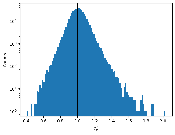
chi2_data = fchi2.read()
is_valid = chi2_data['CONT_valid']

chi2_v = chi2_data[is_valid]['CONT_chi2'] / chi2_data[is_valid]['CONT_dof']

plt.hist(chi2_v, bins=100)
plt.axvline(1, c='k')
plt.xlabel(r"$\chi^2_\nu$")
plt.ylabel("Counts")
plt.yscale("log")
plt.show()
Now let us investigate the attributes.fits file, which contains the mean continuum in CONT-i extensions, stacked fluxes in observed frame in STACKED_FLUX-i, in rest-frame in STACKED_FLUX_RF-i extensions, and varlss-eta values in VAR_FUNC-i extenstions for all iterations.
fattr = fitsio.FITS(f"{output_delta_folder}/attributes.fits")
fattr
Output:
file: Delta-co1/attributes.fits
extnum hdutype         hduname[v]
0      IMAGE_HDU
1      BINARY_TBL      CONT-1
2      BINARY_TBL      STACKED_FLUX-1
3      BINARY_TBL      STACKED_FLUX_RF-1
4      BINARY_TBL      VAR_FUNC-1
5      BINARY_TBL      CONT-2
6      BINARY_TBL      STACKED_FLUX-2
7      BINARY_TBL      STACKED_FLUX_RF-2
8      BINARY_TBL      VAR_FUNC-2
9      BINARY_TBL      CONT-3
10     BINARY_TBL      STACKED_FLUX-3
11     BINARY_TBL      STACKED_FLUX_RF-3
12     BINARY_TBL      VAR_FUNC-3
13     BINARY_TBL      CONT-4
14     BINARY_TBL      STACKED_FLUX-4
15     BINARY_TBL      STACKED_FLUX_RF-4
16     BINARY_TBL      VAR_FUNC-4
17     BINARY_TBL      CONT-5
18     BINARY_TBL      STACKED_FLUX-5
19     BINARY_TBL      STACKED_FLUX_RF-5
20     BINARY_TBL      VAR_FUNC-5
21     BINARY_TBL      CONT-6
22     BINARY_TBL      STACKED_FLUX-6
23     BINARY_TBL      STACKED_FLUX_RF-6
24     BINARY_TBL      VAR_FUNC-6
25     BINARY_TBL      CONT
26     BINARY_TBL      STACKED_FLUX
27     BINARY_TBL      STACKED_FLUX_RF
28     BINARY_TBL      VAR_FUNC
29     BINARY_TBL      VAR_STATS
fattr['VAR_STATS']
Output:
file: Delta-co1/attributes.fits
extension: 29
type: BINARY_TBL
extname: VAR_STATS
rows: 2500
column info:
  wave                f8
  var_pipe            f8
  e_var_pipe          f8
  var_delta           f8
  e_var_delta         f8
  mean_delta          f8
  var2_delta          f8
  num_pixels          i8
  num_qso             i8
  cov_var_delta       f8  array[100]
Note you will have cov_var_delta only if you ran qsonic-fit with --var-use-cov option.
fattr['VAR_STATS'].read_header()
Output:
XTENSION= 'BINTABLE'           / binary table extension
BITPIX  =                    8 / 8-bit bytes
NAXIS   =                    2 / 2-dimensional binary table
NAXIS1  =                  872 / width of table in bytes
NAXIS2  =                 2500 / number of rows in table
PCOUNT  =                    0 / size of special data area
GCOUNT  =                    1 / one data group (required keyword)
TFIELDS =                   10 / number of fields in each row
TTYPE1  = 'wave'               / label for field   1
TFORM1  = 'D'                  / data format of field: 8-byte DOUBLE
TTYPE2  = 'var_pipe'           / label for field   2
TFORM2  = 'D'                  / data format of field: 8-byte DOUBLE
TTYPE3  = 'e_var_pipe'         / label for field   3
TFORM3  = 'D'                  / data format of field: 8-byte DOUBLE
TTYPE4  = 'var_delta'          / label for field   4
TFORM4  = 'D'                  / data format of field: 8-byte DOUBLE
TTYPE5  = 'e_var_delta'        / label for field   5
TFORM5  = 'D'                  / data format of field: 8-byte DOUBLE
TTYPE6  = 'mean_delta'         / label for field   6
TFORM6  = 'D'                  / data format of field: 8-byte DOUBLE
TTYPE7  = 'var2_delta'         / label for field   7
TFORM7  = 'D'                  / data format of field: 8-byte DOUBLE
TTYPE8  = 'num_pixels'         / label for field   8
TFORM8  = 'K'                  / data format of field: 8-byte INTEGER
TTYPE9  = 'num_qso'            / label for field   9
TFORM9  = 'K'                  / data format of field: 8-byte INTEGER
TTYPE10 = 'cov_var_delta'      / label for field  10
TFORM10 = '100D'               / data format of field: 8-byte DOUBLE
EXTNAME = 'VAR_STATS'          / name of this binary table extension
MINNPIX =                  500 /
MINNQSO =                   50 /
MINSNR  =                    0 /
MAXSNR  =                  100 /
WAVE1   =               3660.0 /
WAVE2   =               6540.0 /
NWBINS  =                   25 /
IVAR1   =                 0.05 /
IVAR2   =              10000.0 /
NVARBINS=                  100 /
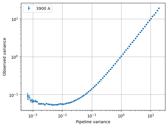
Plotting var_pipe vs var_obs for a wavelength bin
hdr = fattr['VAR_STATS'].read_header()
nwbins = hdr['NWBINS']
nvarbins = hdr['NVARBINS']
min_nqso = hdr['MINNQSO']
min_npix = hdr['MINNPIX']
del hdr

var_stats_data = fattr['VAR_STATS'].read().reshape(nwbins, nvarbins)

# Pick a wavelength bin to plot
iw = 2
dat = var_stats_data[iw]
valid = (dat['num_qso'] >= min_nqso) & (dat['num_pixels'] >= min_npix)
dat = dat[valid]

plt.errorbar(
    dat['var_pipe'], dat['var_delta'], dat['e_var_delta'],
    fmt='.', alpha=1, label=f"{np.mean(dat['wave']):.0f} A")
plt.xlabel("Pipeline variance")
plt.ylabel("Observed variance")
plt.xscale("log")
plt.yscale("log")
plt.grid()
plt.legend()
plt.show()
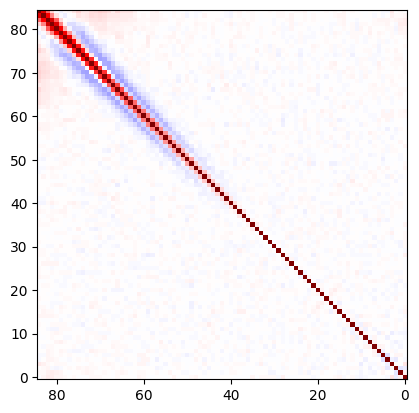
Plot covariance between these points
cov = dat['cov_var_delta'][:, valid]
norm = np.sqrt(cov.diagonal())
plt.imshow(cov / np.outer(norm, norm), vmin=-1, vmax=1, cmap=plt.cm.seismic)
plt.gca().invert_yaxis()
plt.gca().invert_xaxis()
plt.show()
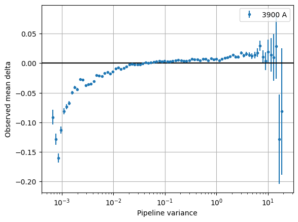
Plot var_pipe vs mean_delta
plt.errorbar(
    dat['var_pipe'], dat['mean_delta'], np.sqrt(dat['var_delta'] / dat['num_pixels']),
    fmt='.', alpha=1, label=f"{np.mean(dat['wave']):.0f} A")
plt.xlabel("Pipeline variance")
plt.ylabel("Observed mean delta")
plt.xscale("log")
plt.grid()
plt.axhline(0, c='k')
plt.legend()
plt.show()
Running qsonic-calib
qsonic-calib calculates var_lss and eta terms for a given set of deltas. This script does not perform continuum fitting, and so it enables fast calculations of var_lss and eta for data SNR splits, parameter variations in wavelength and variance binning. Using the same OUTPUT_FOLDER that we saved our deltas, you can run qsonic-calib for SNR>2 deltas with 200 variance bins as follows:
srun -n 16 -c 2 qsonic-calib \
-i OUTPUT_FOLDER -o OUTPUT_FOLDER \
--nvarbins 200 --var-use-cov --min-snr 2 \
--wave1 3600 --wave2 5500 \
--forest-w1 1040 --forest-w2 1200
Reading spectra
Here’s an example code snippet to use IO interface following the EDR instructions above. See below for a step by step tutorial.
import numpy as np
import qsonic.catalog
import qsonic.io

fname_catalog = "QSO_cat_fuji_healpix_only_qso_targets_sv3_fix.fits"
indir = "${EDR_DIRECTORY}/spectro/redux/fuji/healpix"
arms = ['B', 'R']
is_mock = False
skip_resomat = True

# Setup reader function
readerFunction = qsonic.io.get_spectra_reader_function(
    indir, arms, is_mock, skip_resomat,
    read_true_continuum=False, is_tile=False)

w1 = 3600.
w2 = 6000.
fw1 = 1050.
fw2 = 1180.

catalog = qsonic.catalog.read_quasar_catalog(fname_catalog, is_mock=is_mock)

# Group into unique pixels
unique_pix, s = np.unique(catalog['HPXPIXEL'], return_index=True)
split_catalog = np.split(catalog, s[1:])

# You can parallelize this such that each process reads a healpix.
# e.g., pool.map(parallel_reading, split_catalog)
for hpx_cat in split_catalog:
    healpix = hpx_cat['HPXPIXEL'][0]

    spectra_by_hpx = readerFunction(hpx_cat)

    # Do stuff with spectra in this healpix
    ...
Simple coadd showcase
An empty notebook can be found in the GitHub repo under docs/nb/simple_coadd_showcase.ipynb or downloaded here.
For this example, we are going to read all arms (B, R, Z), but will not read the resolution matrix.
import numpy as np
import matplotlib.pyplot as plt

import qsonic.catalog
import qsonic.io

fname_catalog = "QSO_cat_fuji_healpix_only_qso_targets_sv3_fix.fits"
indir = "${EDR_DIRECTORY}/spectro/redux/fuji/healpix"
arms = ['B', 'R', 'Z']
is_mock = False
skip_resomat = True

# Setup reader function
readerFunction = qsonic.io.get_spectra_reader_function(
    indir, arms, is_mock, skip_resomat,
    read_true_continuum=False, is_tile=False)
First, we read the catalog. Since qsonic sorts this the catalog by
HPXPIXEL, we can find the unique healpix values and split the catalog
into healpix groups. For example purposes, we are picking a single healpix and
reading all the quasar spectra in that file.
catalog = qsonic.catalog.read_quasar_catalog(fname, is_mock=is_mock)

# Group into unique pixels
unique_pix, s = np.unique(catalog['HPXPIXEL'], return_index=True)
split_catalog = np.split(catalog, s[1:])

# Pick one healpix to illustrate
hpx_cat = split_catalog[1]
healpix = hpx_cat['HPXPIXEL'][0]

spectra_by_hpx = readerFunction(hpx_cat)

print(f"There are {len(spectra_by_hpx)} spectra in healpix {healpix}.")
There are 71 spectra in healpix 9145.
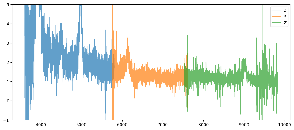
Plot one spectrum
Let’s investigate one spectrum. Wavelength, flux and inverse variance are stored as dictionaries similar to desispec.spectra.Spectra.
spec = spectra_by_hpx[3]
print(spec.wave)
print(spec.flux)
{'B': array([3600. , 3600.8, 3601.6, ..., 5798.4, 5799.2, 5800. ]),
 'R': array([5760. , 5760.8, 5761.6, ..., 7618.4, 7619.2, 7620. ]),
 'Z': array([7520. , 7520.8, 7521.6, ..., 9822.4, 9823.2, 9824. ])}
{'B': array([0.16013083, 2.1076498 , 6.495008  , ..., 2.2043223 , 1.6862453 ,
    1.8163666 ], dtype=float32),
 'R': array([-1.287594  ,  1.731283  ,  0.62619126, ...,  0.9037217 ,
    1.3648763 ,  1.652868  ], dtype=float32),
 'Z': array([0.83304965, 1.031328  , 1.6591258 , ..., 0.81355166, 1.0301682 ,
    1.0923132 ], dtype=float32)}
plt.figure(figsize=(12, 5))
for arm, wave_arm in spec.wave.items():
    plt.plot(wave_arm, spec.flux[arm], label=arm, alpha=0.7)
plt.legend()
plt.ylim(-1, 5)
plt.show()
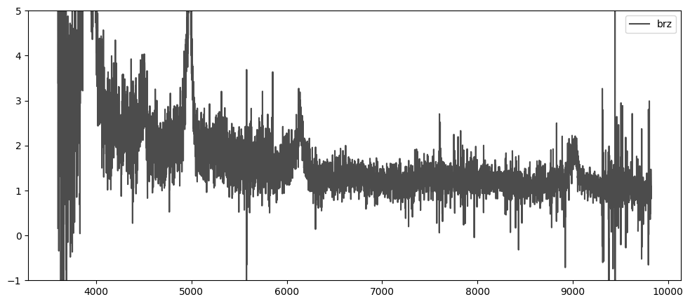
Plot coadded spectrum
Now, we coadd the arms using inverse variance and replot. The spectrum
attributes will still be dictionaries with a single key brz no
matter which arms are used to coadd.
spec.simple_coadd()
print(spec.wave)
print(spec.flux)
{'brz': array([3600. , 3600.8, 3601.6, ..., 9822.4, 9823.2, 9824. ])}
{'brz': array([0.16013082, 2.10764978, 6.49500805, ..., 0.81355166, 1.03016822,
    1.0923132 ])}
plt.figure(figsize=(12, 5))
for arm, wave_arm in spec.wave.items():
    plt.plot(wave_arm, spec.flux[arm], label=arm, alpha=0.7, c='k')
plt.legend()
plt.ylim(-1, 5)
plt.show()